Posterior Predictive Checking with predictCheckR

Introduction

Posterior predictive checking (PPC) is a principled, simulation-based technique for assessing Bayesian model fit. Rather than relying solely on likelihood-based information criteria, PPC asks a direct question:

If the model is correct, would it generate data that look like the data we actually observed?

The Posterior Predictive Distribution

Given a Bayesian model with likelihood $p(y \mid \theta)$ and prior $p(\theta)$ , inference yields the posterior $p(\theta \mid y) \propto p(y \mid \theta)\, p(\theta)$ . The posterior predictive distribution for a future — or hypothetically replicated — outcome $y^{rep}$ is

$p(y^{rep} \mid y) = \int p(y^{rep} \mid \theta)\, p(\theta \mid y)\, d\theta.$

In practice the integral is approximated by Monte Carlo averaging over $S$ posterior draws $\theta^{(1)}, \ldots, \theta^{(S)}$ :

$p(y^{rep} \mid y) \approx \frac{1}{S} \sum_{s=1}^{S} p\!\left(y^{rep} \mid \theta^{(s)}\right).$

Each draw $y^{rep(s)}$ is a complete replicated dataset of the same size as $y$ . The collection $\{y^{rep(s)}\}_{s=1}^{S}$ forms the posterior predictive ensemble that is used for visual and numerical diagnostics.

Predictive Discrepancy Statistics

A scalar test statistic $T(\cdot)$ summarises some property of a dataset (e.g. the mean, standard deviation, or a tail quantile). The Bayesian $p$ -value for $T$ is

$p_B = \Pr\!\left(T(y^{rep}) \geq T(y) \mid y\right) \approx \frac{1}{S}\sum_{s=1}^{S} \mathbf{1}\!\left[T(y^{rep(s)}) \geq T(y)\right].$

A value of $p_B \approx 0.5$ indicates that the model is well-calibrated with respect to $T$ . Extreme values ( $p_B < 0.05$ or $p_B > 0.95$ ) flag potential misfit.

Package Setup

Install predictCheckR from GitHub (once published) or load it from the source directory during development:

library(predictCheckR)
library(ggplot2)

The Example Dataset

predictCheckR ships with example_data, a small simulated regression dataset generated from the model

$x_i \sim \mathcal{N}(0, 1), \qquad y_i = 2 + 3 x_i + \varepsilon_i, \qquad \varepsilon_i \sim \mathcal{N}(0, 1), \qquad i = 1, \ldots, 100.$

data(example_data)
head(example_data)
#>            x        y
#> 1  0.9819694 7.154570
#> 2  0.4687150 3.846278
#> 3 -0.1079713 2.719252
#> 4 -0.2128782 1.487042
#> 5  1.1580985 4.209046
#> 6  1.2923548 6.251425

ggplot(example_data, aes(x = x, y = y)) +
  geom_point(alpha = 0.6, colour = "steelblue") +
  geom_smooth(method = "lm", se = TRUE, colour = "grey30",
              fill = "grey80", linewidth = 0.8) +
  labs(
    title    = "Example Regression Dataset",
    subtitle = "True model: y = 2 + 3x + N(0,1)",
    x        = "Predictor  x",
    y        = "Response  y"
  ) +
  theme_ppc()
#> `geom_smooth()` using formula = 'y ~ x'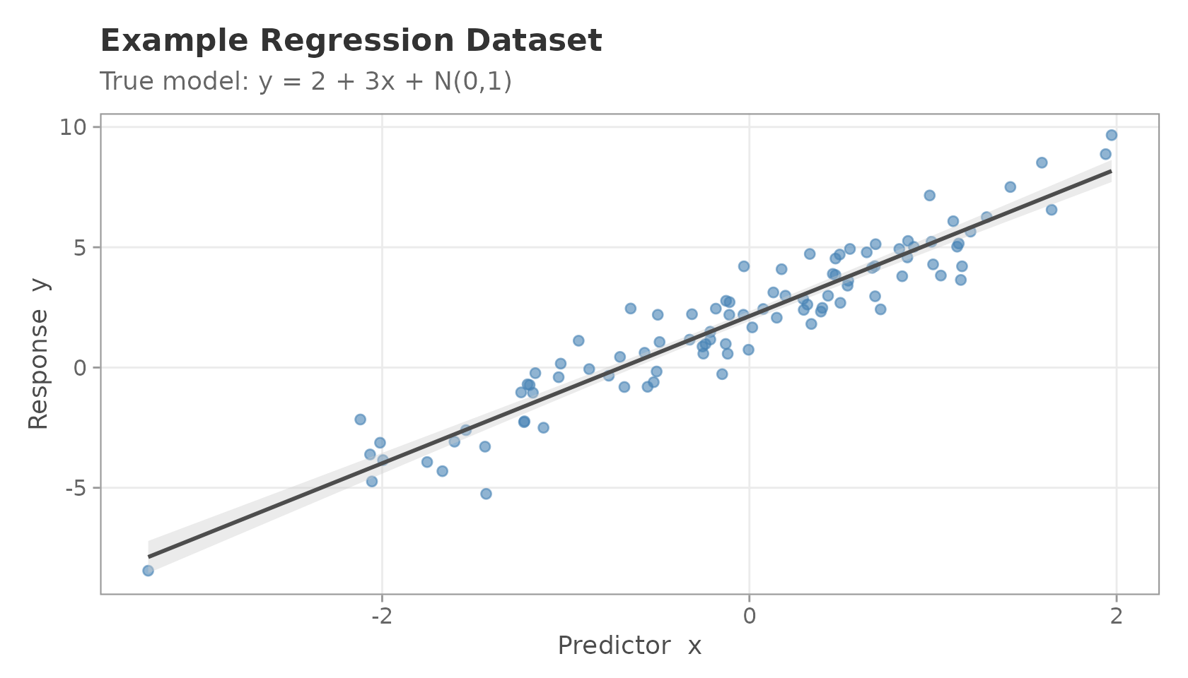

Scatter plot of the example regression dataset.

Generating Fake Posterior Draws

In a real analysis, posterior draws would come from a sampler such as rstan or brms. Here we simulate draws directly to keep the vignette self-contained.

Suppose we have obtained $S = 400$ posterior samples of the intercept $\alpha$ and slope $\beta$ . We centre the draws on the true values but add realistic posterior uncertainty.

set.seed(101)
S <- 400   # posterior iterations
n <- nrow(example_data)

# Simulate posterior draws: alpha ~ N(2, 0.15^2), beta ~ N(3, 0.12^2)
alpha_draws <- rnorm(S, mean = 2.0, sd = 0.15)
beta_draws  <- rnorm(S, mean = 3.0, sd = 0.12)
sigma_draws <- abs(rnorm(S, mean = 1.0, sd = 0.08))  # residual SD draws

# Posterior draws matrix (S x 2): columns are [alpha, beta]
posterior_draws <- cbind(intercept = alpha_draws, slope = beta_draws)

# Design matrix (n x 2): [1, x]
X <- cbind(1, example_data$x)

dim(posterior_draws)
#> [1] 400   2
dim(X)
#> [1] 100   2

Generating Posterior Predictive Samples

simulate_ppc() takes the $S \times P$ draws matrix and an optional design matrix to produce the $S \times n$ replicated data matrix.

y_rep <- simulate_ppc(
  posterior_draws = posterior_draws,
  X               = X,
  family          = "gaussian",
  sigma_posterior = sigma_draws
)

dim(y_rep)   # 400 rows (draws) x 100 columns (observations)
#> [1] 400 100

Each row of y_rep is one plausible dataset that the model could have generated.

Running Posterior Predictive Diagnostics

ppc_diagnostics() computes several scalar discrepancy statistics and returns an S3 object with a dedicated print method.

y_obs <- example_data$y

diag_result <- ppc_diagnostics(y_obs = y_obs, y_rep = y_rep)
print(diag_result)
#> 
#> -- Posterior Predictive Diagnostics (predictCheckR) --
#> 
#>   Draws  : 400
#>   Obs    : 100
#> 
#>   Discrepancy Statistics:
#>     Mean difference        : -0.1263
#>     Variance difference    : -0.4878
#>     Bayesian p-value       : 0.2475
#>     RMSE (pred vs. obs)    : 1.025
#>     Coverage (95% CI)      : 0.94

Interpreting the output:

Statistic	Interpretation
Mean difference	Should be close to 0.
Variance difference	Should be close to 0.
Bayesian $p$ -value	Values near 0.5 indicate calibration.
RMSE	Lower is better; reflects point-prediction accuracy.
Coverage (95 % CI)	Should be near 0.95 for a well-calibrated model.

Visualisation

Density Overlay

The density overlay is the workhorse visualisation for PPC. It superimposes the kernel density estimate of $y^{obs}$ (dark line) over a random subsample of $y^{rep}$ densities (light lines).

plot_ppc_overlay(
  y_obs     = y_obs,
  y_rep     = y_rep,
  n_samples = 50
)

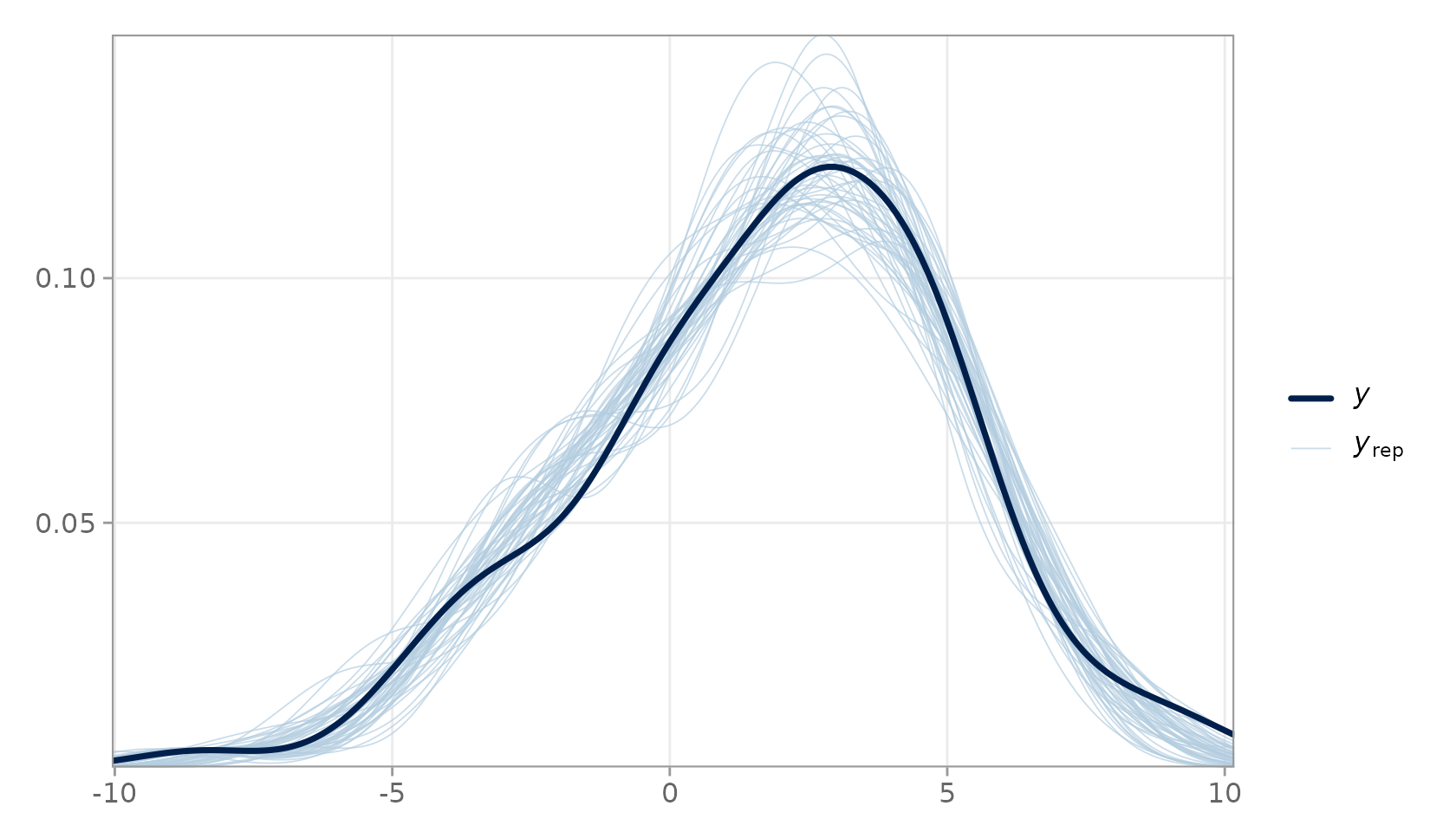
PPC density overlay. The dark line is the observed data; light lines are 50 random posterior predictive replicates.

Close agreement between the dark and light lines indicates that the model reproduces the marginal distribution of the response faithfully.

Test-Statistic Distribution

plot_ppc_stat() shows the distribution of $T(y^{rep})$ across all draws as a histogram, with a vertical line for $T(y^{obs})$ .

plot_ppc_stat(y_obs = y_obs, y_rep = y_rep, stat = "mean")
#> Note: in most cases the default test statistic 'mean' is too weak to detect anything of interest.
#> `stat_bin()` using `bins = 30`. Pick better value `binwidth`.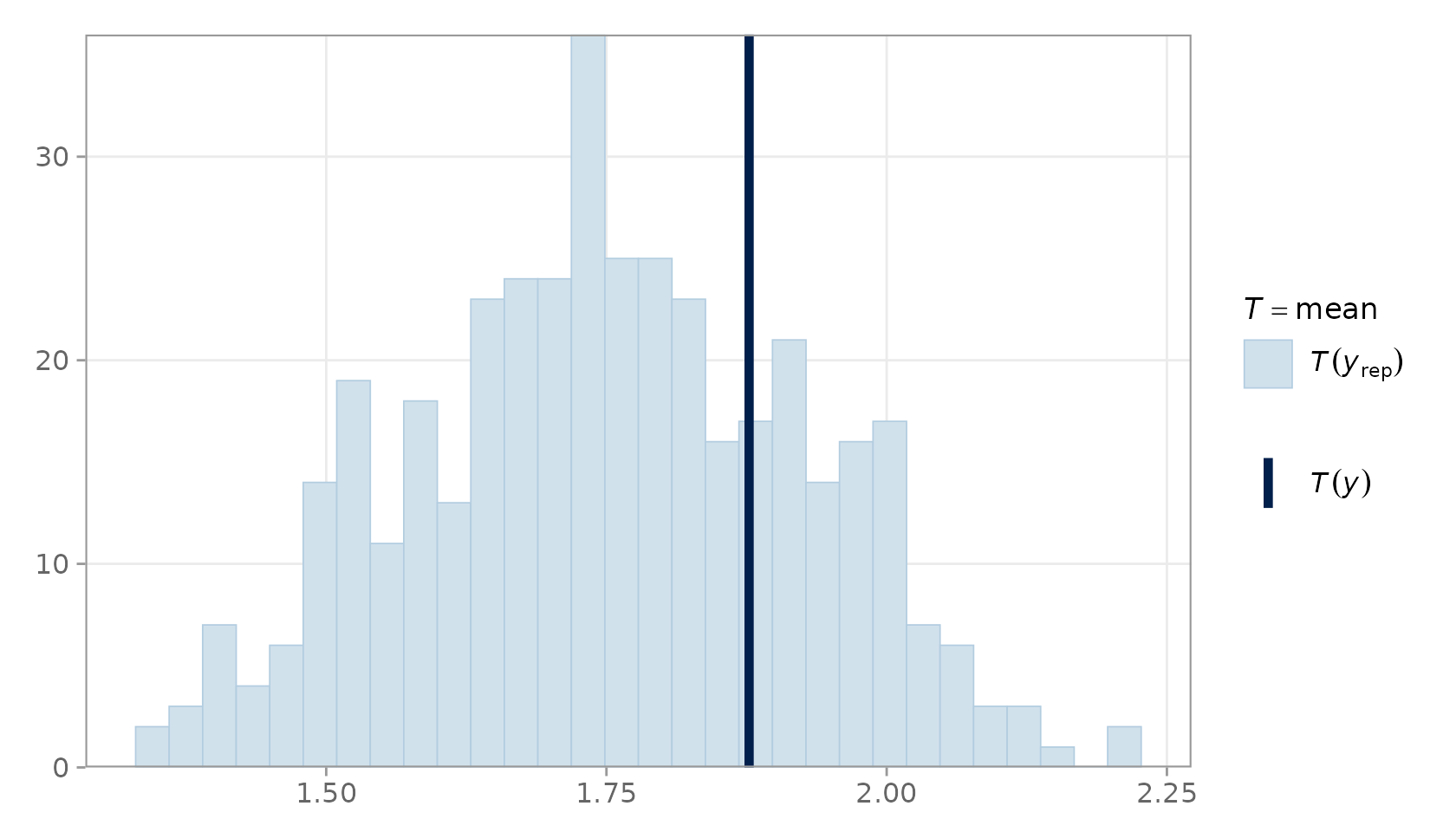

PPC statistic plot for the mean.

plot_ppc_stat(y_obs = y_obs, y_rep = y_rep, stat = "sd")
#> `stat_bin()` using `bins = 30`. Pick better value `binwidth`.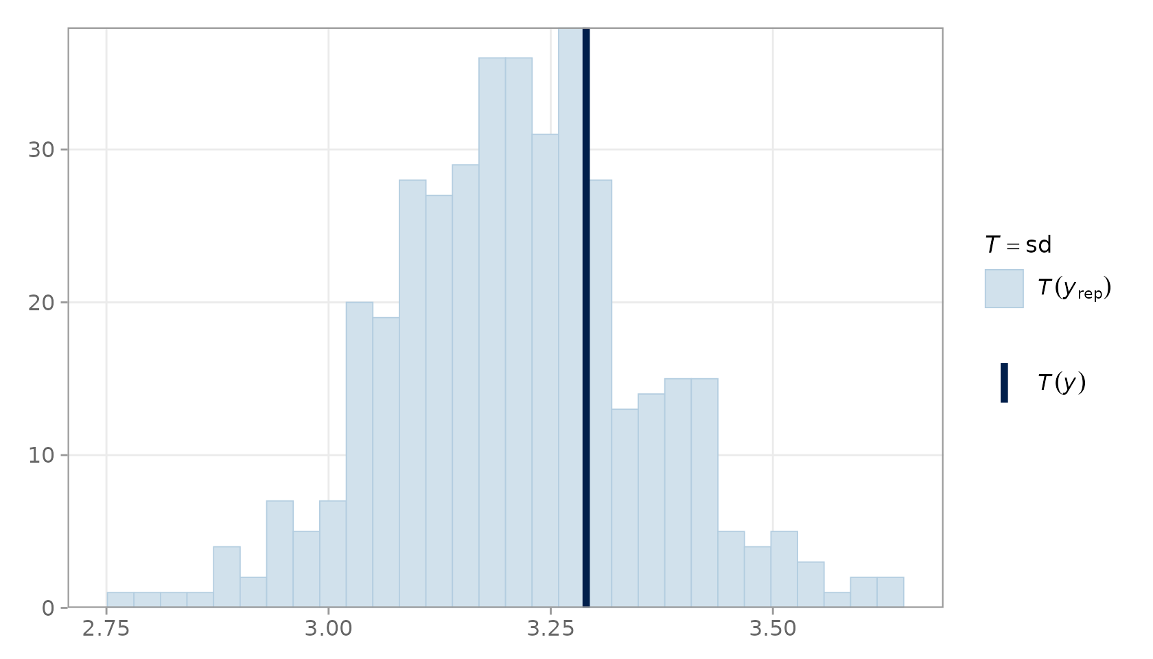

PPC statistic plot for the standard deviation.

The vertical line (observed statistic) should fall well within the histogram mass when the model is well-specified.

Model Comparison

compare_models_ppc() produces a side-by-side table of predictive performance metrics for two competing models, making it straightforward to assess which model better describes the data.

# Mis-specified model: draws centred on a shifted mean
set.seed(202)
posterior_draws_bad <- cbind(
  intercept = rnorm(S, mean = 4.0, sd = 0.15),   # wrong intercept
  slope     = rnorm(S, mean = 3.0, sd = 0.12)
)

y_rep_bad <- simulate_ppc(
  posterior_draws = posterior_draws_bad,
  X               = X,
  family          = "gaussian",
  sigma_posterior = sigma_draws
)

compare_models_ppc(
  y_obs       = y_obs,
  y_rep1      = y_rep,
  y_rep2      = y_rep_bad,
  model_names = c("Correct Model", "Shifted Intercept")
)
#>               metric Correct Model Shifted Intercept diff_m1_minus_m2
#> 1               RMSE      1.024788          2.120722        -1.095933
#> 2                MAE      0.828283          1.882697        -1.054414
#> 3 Pred. Variance Gap      9.792874          9.770498         0.022376

The correctly-specified model should show lower RMSE and MAE, and a predictive variance gap close to zero.

Conclusion and Interpretation

Posterior predictive checking provides a transparent, simulation-based window into model adequacy. The predictCheckR workflow consists of four steps:

Fit a Bayesian model and extract $S$ posterior draw vectors.
Simulate posterior predictive replicates with simulate_ppc().
Diagnose discrepancies with ppc_diagnostics().
Visualise with plot_ppc_overlay() and plot_ppc_stat().

When the model is well-specified, replicated data should be statistically indistinguishable from the observed data. Systematic departures — heavy tails, multimodality, bias in a test statistic — point directly to the aspects of the data-generating process that the model fails to capture.

Session Information

sessionInfo()
#> R version 4.5.3 (2026-03-11)
#> Platform: x86_64-pc-linux-gnu
#> Running under: Ubuntu 24.04.4 LTS
#> 
#> Matrix products: default
#> BLAS:   /usr/lib/x86_64-linux-gnu/openblas-pthread/libblas.so.3 
#> LAPACK: /usr/lib/x86_64-linux-gnu/openblas-pthread/libopenblasp-r0.3.26.so;  LAPACK version 3.12.0
#> 
#> locale:
#>  [1] LC_CTYPE=C.UTF-8       LC_NUMERIC=C           LC_TIME=C.UTF-8       
#>  [4] LC_COLLATE=C.UTF-8     LC_MONETARY=C.UTF-8    LC_MESSAGES=C.UTF-8   
#>  [7] LC_PAPER=C.UTF-8       LC_NAME=C              LC_ADDRESS=C          
#> [10] LC_TELEPHONE=C         LC_MEASUREMENT=C.UTF-8 LC_IDENTIFICATION=C   
#> 
#> time zone: UTC
#> tzcode source: system (glibc)
#> 
#> attached base packages:
#> [1] stats     graphics  grDevices utils     datasets  methods   base     
#> 
#> other attached packages:
#> [1] ggplot2_4.0.2       predictCheckR_0.1.0
#> 
#> loaded via a namespace (and not attached):
#>  [1] Matrix_1.7-4       bayesplot_1.15.0   gtable_0.3.6       jsonlite_2.0.0    
#>  [5] dplyr_1.2.1        compiler_4.5.3     Rcpp_1.1.1         tidyselect_1.2.1  
#>  [9] stringr_1.6.0      jquerylib_0.1.4    splines_4.5.3      systemfonts_1.3.2 
#> [13] scales_1.4.0       textshaping_1.0.5  yaml_2.3.12        fastmap_1.2.0     
#> [17] lattice_0.22-9     plyr_1.8.9         R6_2.6.1           labeling_0.4.3    
#> [21] generics_0.1.4     knitr_1.51         tibble_3.3.1       desc_1.4.3        
#> [25] bslib_0.10.0       pillar_1.11.1      RColorBrewer_1.1-3 rlang_1.1.7       
#> [29] stringi_1.8.7      cachem_1.1.0       xfun_0.57          fs_2.0.1          
#> [33] sass_0.4.10        S7_0.2.1           cli_3.6.5          pkgdown_2.2.0     
#> [37] withr_3.0.2        magrittr_2.0.4     mgcv_1.9-4         digest_0.6.39     
#> [41] grid_4.5.3         lifecycle_1.0.5    nlme_3.1-168       vctrs_0.7.2       
#> [45] evaluate_1.0.5     glue_1.8.0         farver_2.1.2       ragg_1.5.2        
#> [49] reshape2_1.4.5     rmarkdown_2.31     tools_4.5.3        pkgconfig_2.0.3   
#> [53] htmltools_0.5.9

Utkarsh Pawade

2026-04-04