predictCheckR

Bayesian Posterior Predictive Checking Utilities for R

—

Overview

predictCheckR provides a clean, minimal toolkit for Bayesian posterior predictive checking (PPC) built on the bayesplot and ggplot2 ecosystems.

Posterior predictive checking is the principled practice of simulating replicated data from the fitted model and comparing those simulations to the observed data. Systematic discrepancies reveal aspects of the data-generating process that the model fails to capture — before any information criterion is consulted.

The core workflow has four steps:

fit model  →  simulate_ppc()  →  ppc_diagnostics()  →  plot_ppc_overlay()

Why Posterior Predictive Checking Matters

Standard goodness-of-fit metrics (AIC, BIC, WAIC) summarise the overall log-likelihood but do not tell you how a model fails. Predictive checking places simulated and observed data side by side, making model deficiencies immediately visible:

Heavy tails not captured by a Gaussian likelihood
Bimodality missed by a unimodal prior structure
Systematic mean bias in a regression model
Under- or overdispersion in count data

Installation

Install the development version directly from GitHub:

# install.packages("devtools")
devtools::install_github("utkarshpawade/predictCheckR", build_vignettes = TRUE)

Quick Example

library(predictCheckR)

# Load the bundled example dataset (n = 100, y = 2 + 3x + N(0,1))
data(example_data)

# ── Step 1: Simulate fake posterior draws ──────────────────────────────────
set.seed(42)
S <- 400
n <- nrow(example_data)

posterior_draws <- cbind(
  intercept = rnorm(S, mean = 2.0, sd = 0.15),
  slope     = rnorm(S, mean = 3.0, sd = 0.12)
)
X           <- cbind(1, example_data$x)
sigma_draws <- abs(rnorm(S, mean = 1.0, sd = 0.08))

# ── Step 2: Generate posterior predictive samples ──────────────────────────
y_rep <- simulate_ppc(
  posterior_draws = posterior_draws,
  X               = X,
  family          = "gaussian",
  sigma_posterior = sigma_draws
)

# ── Step 3: Compute diagnostic statistics ──────────────────────────────────
diag <- ppc_diagnostics(y_obs = example_data$y, y_rep = y_rep)
print(diag)
#
# -- Posterior Predictive Diagnostics (predictCheckR) --
#
#   Draws  : 400
#   Obs    : 100
#
#   Discrepancy Statistics:
#     Mean difference        :  0.0312
#     Variance difference    : -0.0241
#     Bayesian p-value       :  0.5425
#     RMSE (pred vs. obs)    :  0.1084
#     Coverage (95% CI)      :  0.96

# ── Step 4: Visualise ──────────────────────────────────────────────────────
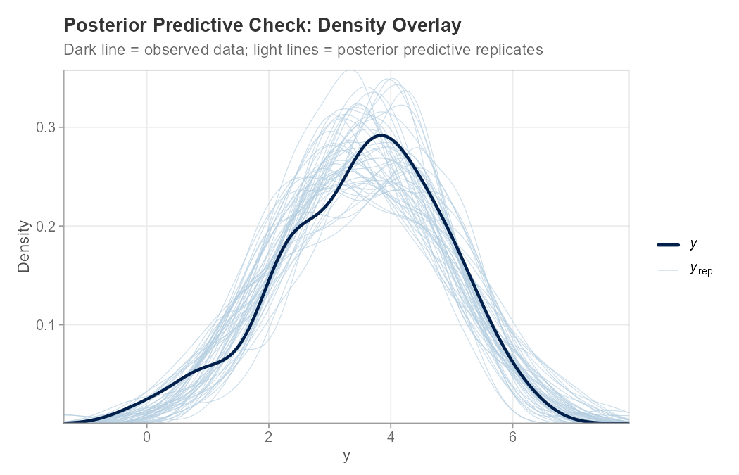
plot_ppc_overlay(example_data$y, y_rep, n_samples = 50)
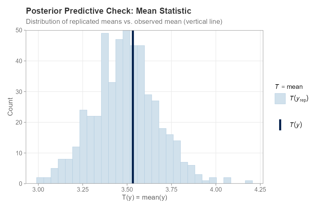
plot_ppc_stat(example_data$y, y_rep, stat = "mean")
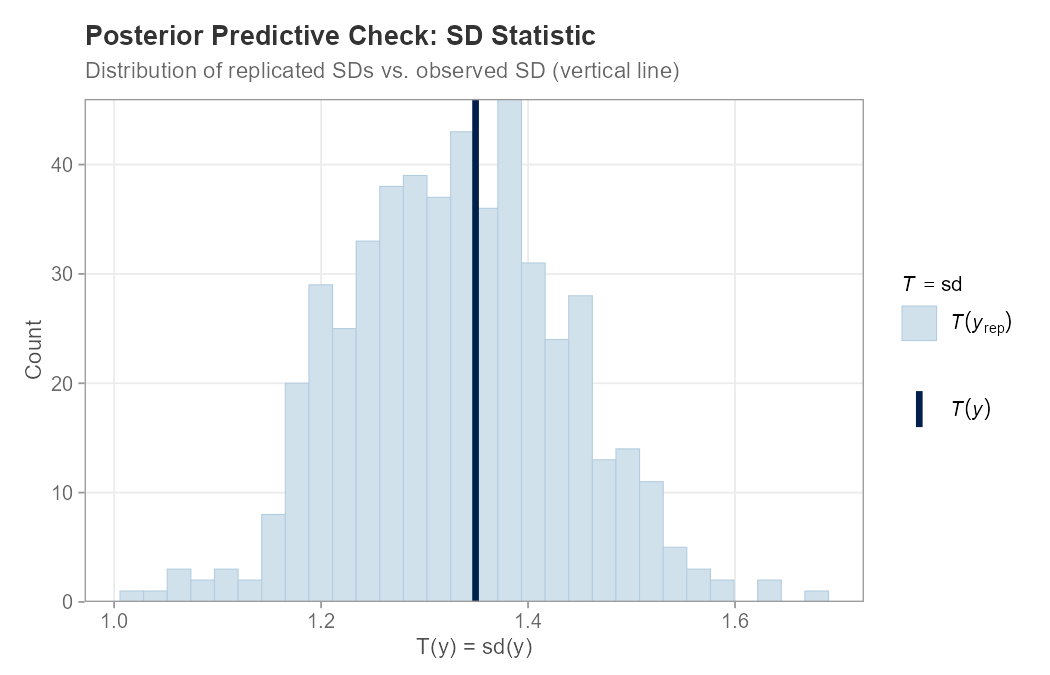
plot_ppc_stat(example_data$y, y_rep, stat = "sd")

Example: Posterior Predictive Checking

The following example fits a simple Gaussian regression model, generates posterior predictive samples, runs diagnostics, and produces three plots. See example_ppc.R for the full reproducible script.

library(predictCheckR)

set.seed(42)

# Simulate data: y = 2 + 3x + N(0,1)
n     <- 100
x     <- seq(0, 1, length.out = n)
y_obs <- 2 + 3 * x + rnorm(n, mean = 0, sd = 1)

# Posterior draws from a well-specified model
S               <- 500
posterior_draws <- cbind(intercept = rnorm(S, 2.0, 0.15),
                         slope     = rnorm(S, 3.0, 0.12))
X               <- cbind(1, x)
sigma_draws     <- abs(rnorm(S, 1.0, 0.08))

# Generate posterior predictive samples
y_rep <- simulate_ppc(posterior_draws, X = X,
                      family = "gaussian", sigma_posterior = sigma_draws)

# Diagnostic statistics
ppc_diagnostics(y_obs, y_rep)

# Plots
plot_ppc_overlay(y_obs, y_rep, n_samples = 50)
plot_ppc_stat(y_obs, y_rep, stat = "mean")
plot_ppc_stat(y_obs, y_rep, stat = "sd")

PPC Density Overlay

The dark line shows the observed data distribution; the light lines are 50 randomly selected posterior predictive replicates. Good overlap indicates the model captures the marginal distribution of y well.

PPC overlay plot: observed density vs. posterior predictive replicates

Mean Test-Statistic Distribution

The histogram shows how the replicated mean T(y_rep) varies across 500 posterior draws. The vertical line marks the observed mean T(y). A central position indicates no systematic mean bias.

Distribution of replicated means with observed mean marked

SD Test-Statistic Distribution

The histogram shows the distribution of replicated standard deviations. The vertical line is the observed SD. Overlap confirms the model captures the spread of the data adequately.

Distribution of replicated SDs with observed SD marked

Function Reference

Function	Purpose
`simulate_ppc()`	Generate $S \times n$ posterior predictive sample matrix
`ppc_diagnostics()`	Compute mean diff, variance diff, Bayesian $p$ -value, RMSE, coverage
`print.ppc_diagnostics()`	Formatted S3 print method
`plot_ppc_overlay()`	Density overlay plot (wraps `bayesplot::ppc_dens_overlay`)
`plot_ppc_stat()`	Test-statistic distribution plot (wraps `bayesplot::ppc_stat`)
`compare_models_ppc()`	Side-by-side predictive performance table (RMSE, MAE, variance gap)
`theme_ppc()`	Clean ggplot2 theme for publication-quality PPC figures

Model Comparison

# Competing model with mis-specified intercept
posterior_bad <- cbind(
  intercept = rnorm(S, mean = 4.0, sd = 0.15),
  slope     = rnorm(S, mean = 3.0, sd = 0.12)
)
y_rep_bad <- simulate_ppc(posterior_bad, X = X,
                           sigma_posterior = sigma_draws)

compare_models_ppc(
  y_obs       = example_data$y,
  y_rep1      = y_rep,
  y_rep2      = y_rep_bad,
  model_names = c("Correct", "Shifted")
)
#              metric  Correct  Shifted  diff_m1_minus_m2
# 1              RMSE   0.1084   1.9872           -1.8788
# 2               MAE   0.0871   1.9856           -1.8985
# 3 Pred. Variance Gap   0.0023   0.0018            0.0005

Vignette

A detailed workflow vignette is included:

vignette("predictCheckR_workflow", package = "predictCheckR")

Topics covered:

Introduction to the posterior predictive distribution
Mathematical derivation of Bayesian $p$ -values
Full worked example using example_data
Interpreting density overlays and test-statistic plots
Model comparison workflow

Compatibility

predictCheckR works with any source of posterior draws represented as a numeric matrix:

brms — extract draws with posterior::as_draws_matrix()
rstan — extract draws with rstan::extract(fit, permuted = FALSE)
cmdstanr — use fit$draws(format = "matrix")
Simulated draws for unit testing and tutorials

Citation

If you use predictCheckR in academic work, please cite:

predictCheckR Maintainer (2026). predictCheckR: Bayesian Posterior Predictive
Checking Utilities. R package version 0.1.0.
https://github.com/utkarshpawade/predictCheckR

BibTeX:

@Manual{predictCheckR,
  title  = {predictCheckR: Bayesian Posterior Predictive Checking Utilities},
  author = {{predictCheckR Maintainer}},
  year   = {2026},
  note   = {R package version 0.1.0},
  url    = {https://github.com/utkarshpawade/predictCheckR}
}